Printing/Drawing Aesara graphs

Aesara provides the functions aesara.printing.pprint() and aesara.printing.debugprint() to print a graph to the terminal before or after compilation. pprint() is more compact and math-like, debugprint() is more verbose. Aesara also provides pydotprint() that creates an image of the function. You can read about them in printing – Graph Printing and Symbolic Print Statement.

Note

When printing Aesara functions, they can sometimes be hard to read. To help with this, you can disable some Aesara rewrites by using the Aesara flag: optimizer_excluding=fusion:inplace. Do not use this during real job execution, as this will make the graph slower and use more memory.

Consider again the logistic regression example:

>>> import numpy as np
>>> import aesara
>>> import aesara.tensor as at
>>> rng = np.random.default_rng(2382)
>>> # Training data
>>> N = 400
>>> feats = 784
>>> D = (rng.standard_normal(N, feats).astype(aesara.config.floatX), rng.integers(size=N,low=0, high=2).astype(aesara.config.floatX))
>>> training_steps = 10000
>>> # Declare Aesara symbolic variables
>>> x = at.matrix("x")
>>> y = at.vector("y")
>>> w = aesara.shared(rng.standard_normal(feats).astype(aesara.config.floatX), name="w")
>>> b = aesara.shared(np.asarray(0., dtype=aesara.config.floatX), name="b")
>>> x.tag.test_value = D[0]
>>> y.tag.test_value = D[1]
>>> # Construct Aesara expression graph
>>> p_1 = 1 / (1 + at.exp(-at.dot(x, w)-b)) # Probability of having a one
>>> prediction = p_1 > 0.5 # The prediction that is done: 0 or 1
>>> # Compute gradients
>>> xent = -y*at.log(p_1) - (1-y)*at.log(1-p_1) # Cross-entropy
>>> cost = xent.mean() + 0.01*(w**2).sum() # The cost to optimize
>>> gw,gb = at.grad(cost, [w,b])
>>> # Training and prediction function
>>> train = aesara.function(inputs=[x,y], outputs=[prediction, xent], updates=[[w, w-0.01*gw], [b, b-0.01*gb]], name = "train")
>>> predict = aesara.function(inputs=[x], outputs=prediction, name = "predict")

Pretty Printing

>>> aesara.printing.pprint(prediction) 
'gt((TensorConstant{1} / (TensorConstant{1} + exp(((-(x \\dot w)) - b)))),
TensorConstant{0.5})'

Debug Print

The pre-compilation graph:

>>> aesara.printing.debugprint(prediction) 
Elemwise{gt,no_inplace} [id A] ''
 |Elemwise{true_divide,no_inplace} [id B] ''
 | |InplaceDimShuffle{x} [id C] ''
 | | |TensorConstant{1} [id D]
 | |Elemwise{add,no_inplace} [id E] ''
 |   |InplaceDimShuffle{x} [id F] ''
 |   | |TensorConstant{1} [id D]
 |   |Elemwise{exp,no_inplace} [id G] ''
 |     |Elemwise{sub,no_inplace} [id H] ''
 |       |Elemwise{neg,no_inplace} [id I] ''
 |       | |dot [id J] ''
 |       |   |x [id K]
 |       |   |w [id L]
 |       |InplaceDimShuffle{x} [id M] ''
 |         |b [id N]
 |InplaceDimShuffle{x} [id O] ''
   |TensorConstant{0.5} [id P]

The post-compilation graph:

>>> aesara.printing.debugprint(predict)  
Elemwise{Composite{GT(scalar_sigmoid((-((-i0) - i1))), i2)}} [id A] ''   4
 |...Gemv{inplace} [id B] ''   3
 | |AllocEmpty{dtype='float64'} [id C] ''   2
 | | |Shape_i{0} [id D] ''   1
 | |   |x [id E]
 | |TensorConstant{1.0} [id F]
 | |x [id E]
 | |w [id G]
 | |TensorConstant{0.0} [id H]
 |InplaceDimShuffle{x} [id I] ''   0
 | |b [id J]
 |TensorConstant{(1,) of 0.5} [id K]

Picture Printing of Graphs

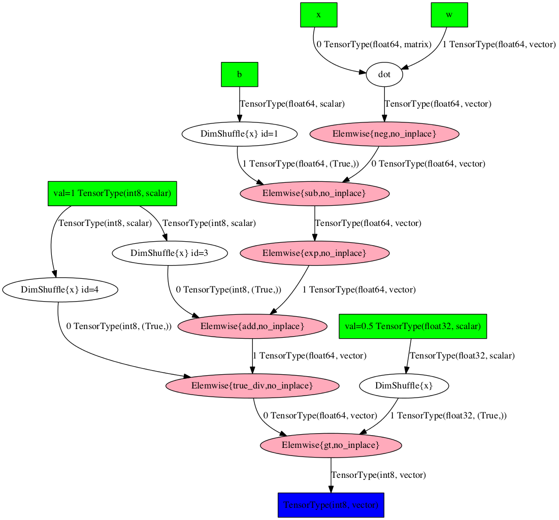
The pre-compilation graph:

>>> aesara.printing.pydotprint(prediction, outfile="logreg_pydotprint_prediction.png", var_with_name_simple=True)  
The output file is available at logreg_pydotprint_prediction.png

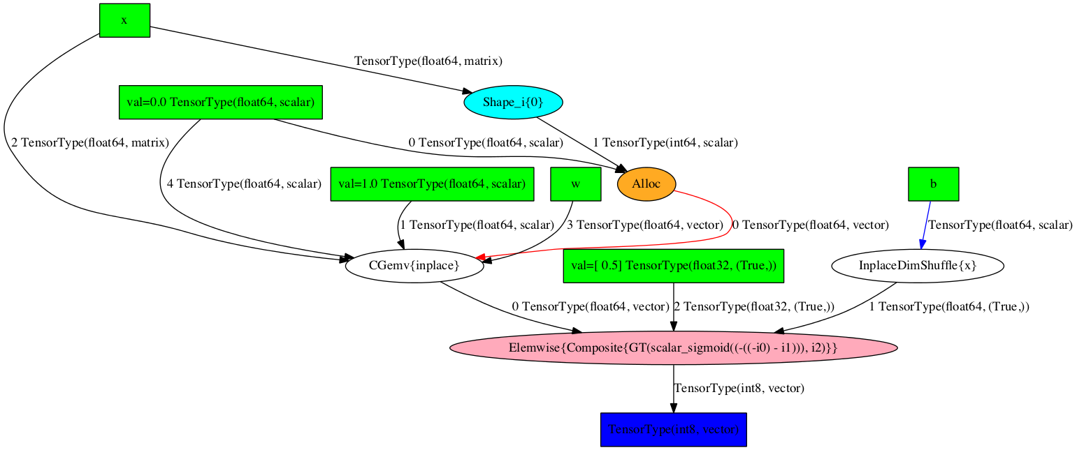
The post-compilation graph:

>>> aesara.printing.pydotprint(predict, outfile="logreg_pydotprint_predict.png", var_with_name_simple=True)  
The output file is available at logreg_pydotprint_predict.png

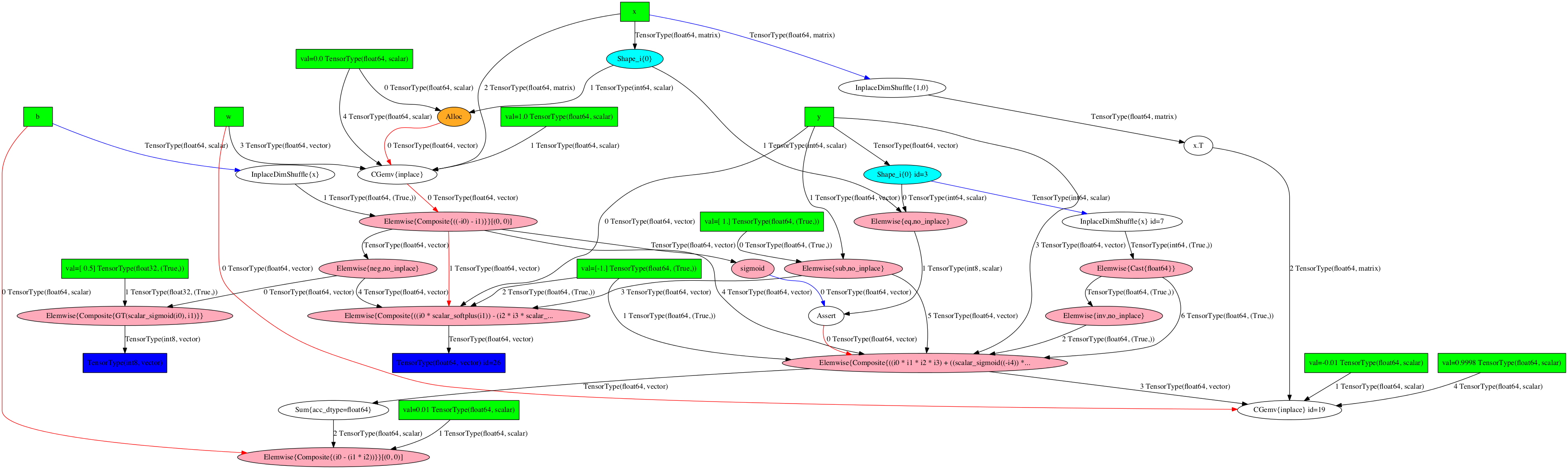
The optimized training graph:

>>> aesara.printing.pydotprint(train, outfile="logreg_pydotprint_train.png", var_with_name_simple=True)  
The output file is available at logreg_pydotprint_train.png

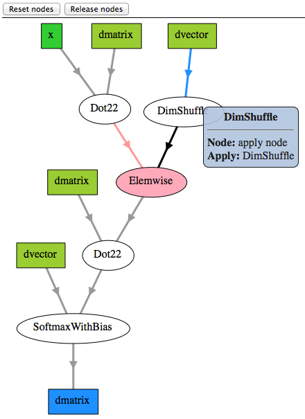
Interactive Graph Visualization

The new d3viz module complements aesara.printing.pydotprint() to visualize complex graph structures. Instead of creating a static image, it generates an HTML file, which allows to dynamically inspect graph structures in a web browser. Features include zooming, drag-and-drop, editing node labels, or coloring nodes by their compute time.

=> d3viz <=